Learning Condition-invariant Scene Representation using UNsupervised Algorithm
When a robot moves in an unknown environment, it needs to create a map and use this map for autonomous localization and navigation. This process is known as Simultaneous Localization and Mapping (SLAM). SLAM is one of the most active areas in robotics research over the past years. In recent years, the SLAM algorithms have been applied in a variety of indoor and outdoor environments.
To build a consistant and less-error map of the environment, it is necessary for a robot to recognize previously visited locations, thsi concept is called as loop-closure detection problem.
A complete visual SLAM system needs several key modules. Among them loop-closure detection is one of the key feature. With the advancements in computer vision, the loop-closure detection problem is frequently addressed in domain of place recognition. Correct loop-closure detection or recognizing the pre-visited places is a very challenging task in complex environments. Hence, robust representation of the scenes is very essential to detect the correct loops as well as to make a more reliable SLAM model.
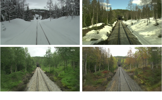
The appearance of a single place can look extremely different in different seasons as demonstrated in Figure 1. Hence it is a very challenging task in computer vision to recognize the same place under different conditions, e.g., in different seasons.

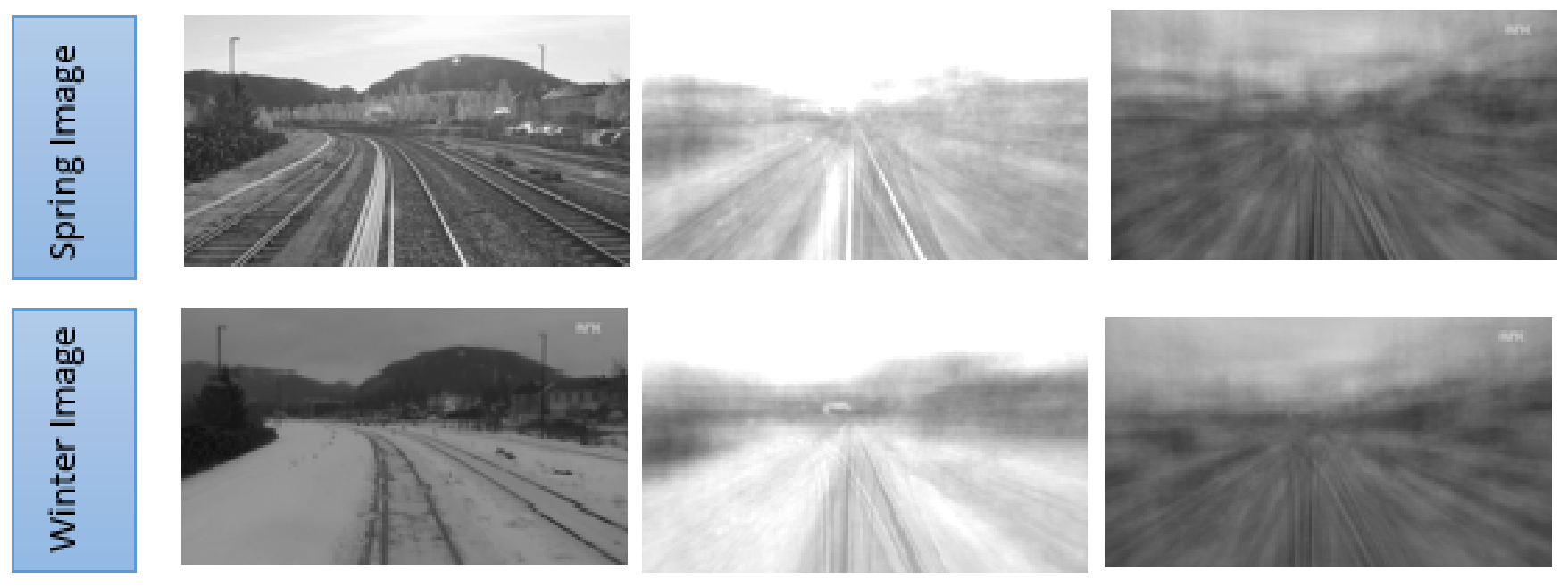
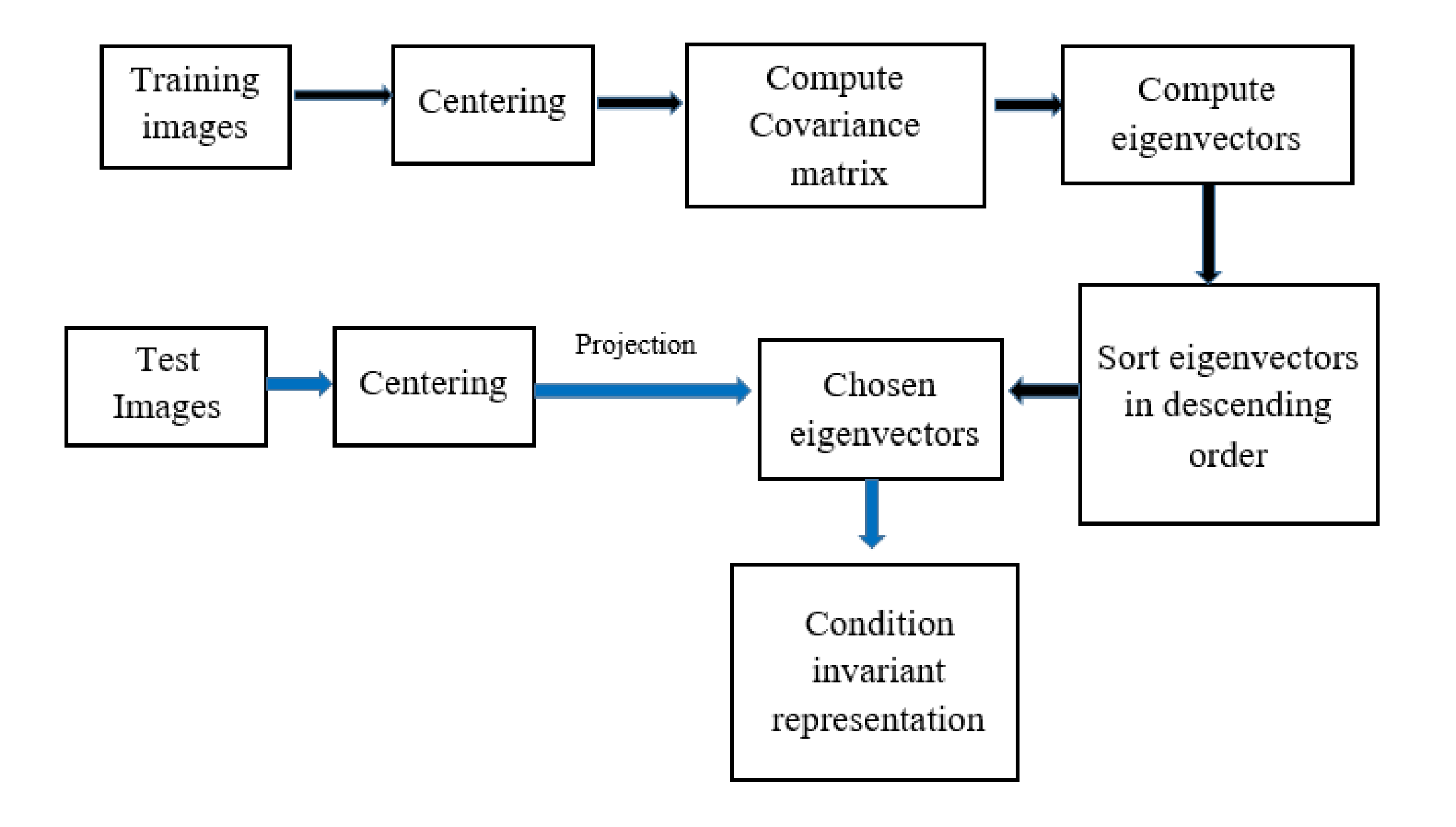
This work is motivated from Supervised and Unsupervised Linear Learning Techniques for Visual Place Recognition in Changing Environments(IEEE Transactions on Robotics 32 (2016)). Their work showed that the PCA can be used to retrieve the robust representations of the scenes by directly applying the PCA to the intensity images. The idea of this algorithm is demonstrated in Figure 2.

Second column: Images are projected on first 100 principal components (PC's)
Third column: Images are projected on second 100 principal components (PC's)

Algorithm is evaluated using the precision-recall curves and the fraction of correct matches. The correct matches are the True Positives (TP), the incorrect matches are the False Positives (FP) and when an algorithm mistakenly discards a correct match, that is labeled as the false negative (FN) match. Since every scene in this dataset has a ground truth match, so there is no true negative (TN), every negative is a false negative (FN).
Precision is defined as the proportion of correct matches to the total number of matches, i.e., correct and incorrect matches. It implies the confidence of the predicted result of an algorithm.
Recall is defined as the proportion of the correct matches to the total number of actual matches. The definition of the precision and recall are given below. \begin{equation} Precision=\frac{TP}{TP+FP} \label{equation_precision} \end{equation} \begin{equation} Recall=\frac{TP}{TP+FN} \label{equation_recall} \end{equation}
High precision refers to the low false positive rate and high recall refers to the low false negative rate.
The precision--recall curves are very useful evaluation measure in the place recognition model (in SLAM we call it In a loop-closure detection model), it is essential to avoid the false positives, because it means two images have been identified as a same place, i.e., it is a loop detection, but in reality, they are from two different locations. This false prediction leads the algorithm to produce the inconsistent map of its surroundings. As the name suggests, the precision--recall curve is a plot of the precision (in $y-axis)$ and recall (in $x-axis$) for the different pairs of the precision and recall values. An ideal error-free model would be the one that reaches $100\%$ precision at $100\%$ recall. The precision--recall curves are generated by varying the number of retrieved or matched images ranging from $1$ to the total number of the test images.
One more evaluation metric has been used, that is the fraction of correct matches. It is defined as the percentage of the number of times the best match the correct loop. $$\text{Fraction of correct matches}=\frac{\text{Number of correct predicted scenes}} {\text{Number of total evaluated scenes}} \times 100 \%$$